Targeted Superlearning🔗

In IPD meta-analysis, univariate moderator analyses are commonly used to identify patients with lower or higher treatment effects. However, their ability to do so may often be limited. The true mechanism that determines how much patients benefit from a psychological intervention is usually unknown; but it will likely depend on a complex interplay of multiple variables that is not easily captured by a simple treatment-covariate interaction. In this sense, even the approaches used in Articles 3 and 4 to model individualized treatment benefits are still fairly restricted: they assume that HTE can be sufficiently explained by one pre-defined parametric model, or a single data-adaptive algorithm.

To this end, in Article 6 (“Estimating Effect Variability Using Targeting Superlearning”), I explore HTE with models that can detect more complex treatment-covariate interactions, based on the targeted superlearning framework (Naimi & Balzer, 2018; Phillips et al., 2023; Polley et al., 2011). I employ this approach in a comprehensive IPD database of preventive intervention trials for subthreshold depression, and examine effects on depressive symptom severity up to 24 months. This section provides some further background and technical details on this methodology, as well as on ancillary software developed as part of the study. The same technical descriptions may also be found, along with other details, in the preregistration of the analysis (Harrer, Sprenger, et al., 2023).

Superlearning (also known as stacked regression; Breiman, 1996) is an ensemble machine learning method that combines multiple prediction algorithms based on their performance in a data set, which is determined using V-fold cross-validation. Prediction algorithms employed in a superlearner typically include both simple linear regression models as well as more “aggressive”, data-adaptive algorithms (e.g., boosting models, support vector machines, neural nets). By combining multiple learners, a superlearner has been shown to asymptotically perform as well as or better than the best-performing individual algorithm included in the framework (“oracle” property; Van der Laan et al., 2007). This method has also been found to be robust across various contexts, and even in very small samples (Montoya et al., 2022; Polley et al., 2011). A key motivation behind superlearning is that the true data-generating process that produced some observed data is often unknown but may be complex, where the framework ensures that the ensemble will converge with the best possible solution for the learning task at hand.

In a treatment setting, the superlearner framework can also be combined with targeted maximum likelihood estimation (TMLE) (Van Der Laan & Rubin, 2006) to estimate optimal dynamic treatment rules (ODTRs) (Murphy, 2003). This ODTR assigns each patient to the optimal (i.e., most effective) treatment based on their pre-test values. This is typically achieved by first estimating the “blip function” (Robins, 2004). This function uses a patient’s set of pre-test values as input and then returns an individualized treatment effect estimate (the “blip”), as derived by the superlearner. While often used as an intermediary step to derive the ODTR, blip distributions themselves can also be of substantive interest (Montoya et al., 2022). For instance, they allow to examine how much patient benefits may vary within a study, who benefits most, and which patients may experience negative effects (i.e., fare worse under treatment than under control).

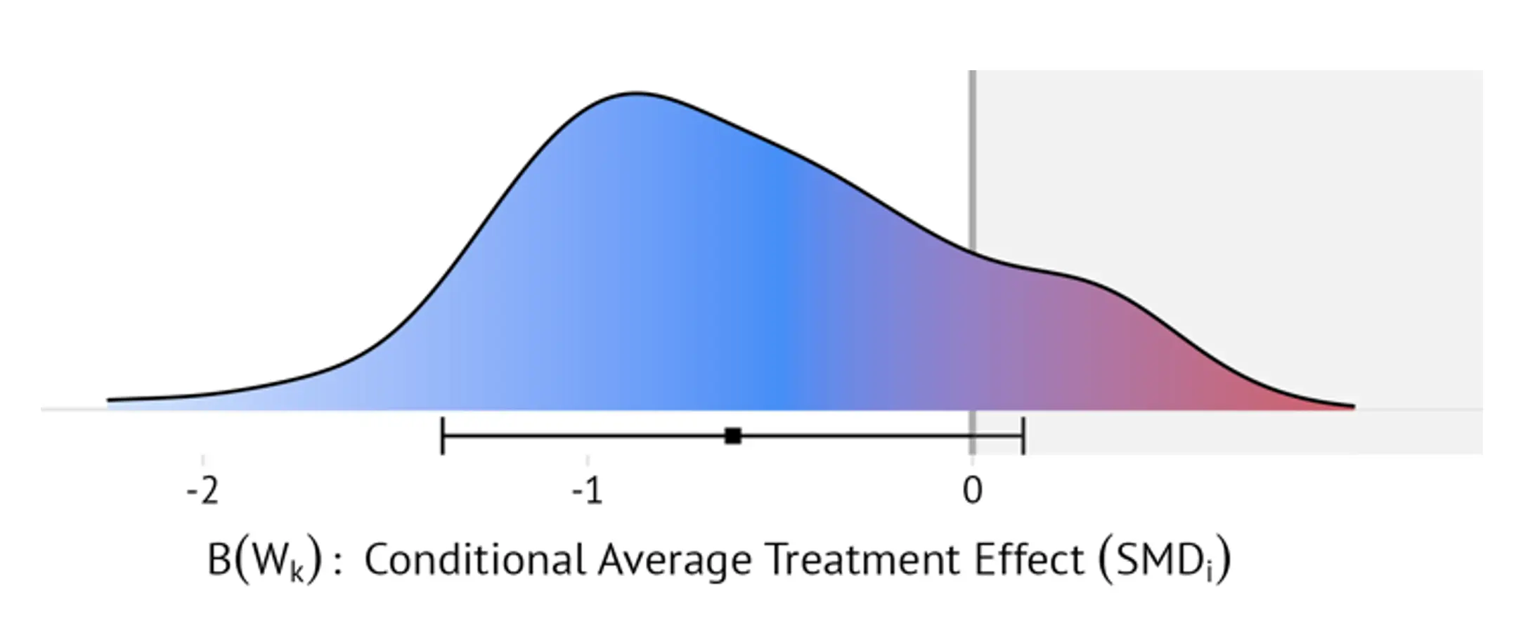
For each study, targeted superlearning was therefore used to estimate the blip distribution across all patients in the trial. Since superlearners were constructed separately for each study, the maximum amount of baseline information included in the IPD database could be used. A broad selection of candidate algorithms was considered within the ensemble, ranging from linear models to more complex machine learning architectures (see Table 1 in Harrer, Sprenger, et al., 2023, for an overview). The distribution of blips, expressed as patient-specific standardized mean differences (SMD), was then presented visually to gauge how strongly individual effects may differ within and across studies. Based on the blips, I also calculated the meta-analytic proportion of patients who experience (i) negative effects, or (ii) only clinically negligible benefits of the preventive interventions (defined as individualized SMDs < 0.24; Cuijpers et al., 2014). Lastly, I constructed an interactive web app that uses the estimated blips to generate individualized meta-analytic effect estimates for specific populations or individuals (e.g., women under the age of 40 with PHQ-9 scores below 6, or any other combination of patient characteristics that were assessed across studies).

I now provide a more technical elaboration of the approach³With slight adaptations, I follow the notation used in Montoya et al. (2022, 2023).. Assume that the individual participant data $D k$ provided by each trial $k$ consists of three components: (i) the vector of baseline covariates $W k$ collected in the trial, (ii) the (binary) treatment $T k$ , and (iii) the outcome of interest $Y k$ ; in our case, patients’ depressive symptom severity. We say that $D k = (W k, T k, Y k)$ with $D k \sim P k$ , where $P k$ is the true data distribution underlying the observed data. Let $M k$ denote a structural causal model of $P k$ (Pearl, 2009), where $U k = (U W k, U T k, U Y k)$ are exogenous (i.e., unobserved) variables. The relationship between the observed and unobserved variables can then be expressed through three structural equations (Díaz Muñoz & van der Laan, 2011; Montoya et al., 2022, 2023):

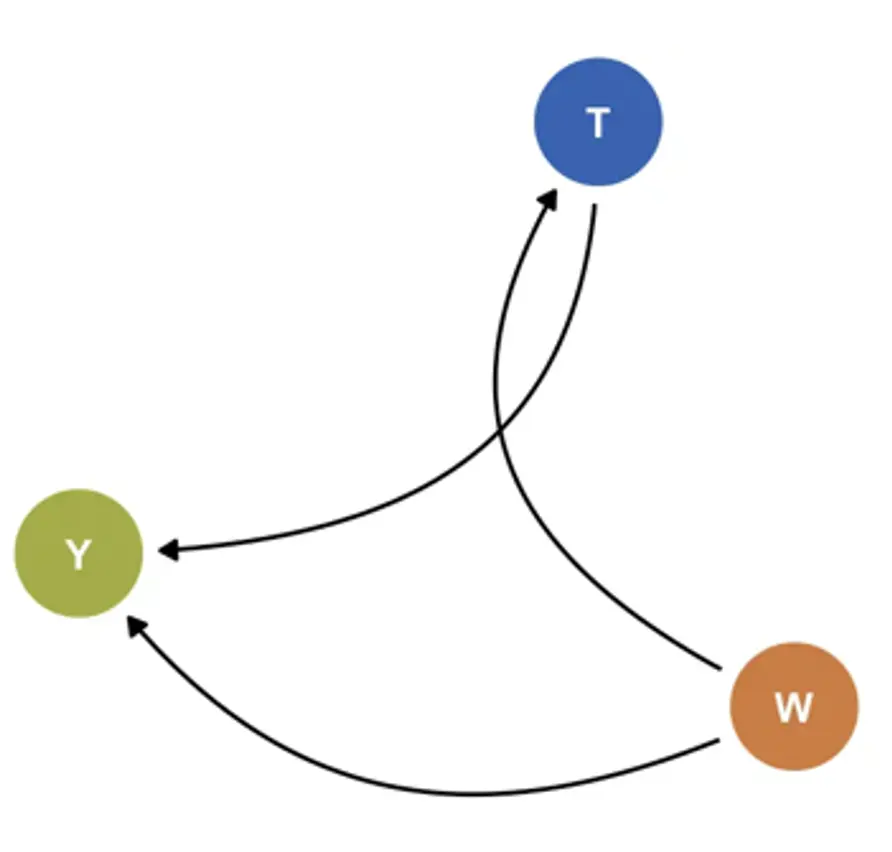
M k = {W k = f W k (U W k) T k = f T k (W k, U T k) Y k = f Y k (W k, T k, U Y k)

(18)

Where $f W k$ and $f Y k$ are unknown functions. According to this model, $Y k$ is a function of the measured covariates $W k$ , unmeasured variables $U Y k$ , and treatment $T k$ . Since $k$ is a randomized trial, it is directly defined by $U T k$ , which has a known distribution: $U T k \sim Bern (p)$ , where $p$ = 0.5 in most cases. Based on this system of data-generating equations, the density of $D k$ can be factorized as:

p (D k) = p W k (W k) g k (T k ∣ W k) p Y k (Y k ∣ T k, W k)

(19)

Where $p W k$ is the density of $W k$ , $g k$ is the treatment assignment mechanism, and $p Y k$ is the conditional density of $Y k$ given $T k$ and $W k$ . Since $k$ is an RCT, $g k$ is known and the positivity assumption $P (min g k (T k = t | W k) > 0) = 1$ with $t \in 0 = control, 1 = treatment$ is known to hold. Also, define $Q k (t, w)$ as the conditional expected value of $Y k$ given $T k$ and $W k$ ; that is $Q k (t, w) = E [Y k | T k = t, W k = w]$ . The blip function $B k (W k)$ can be derived from these conditional expectations by alternatingly setting $t = 1$ and $t = 0$ while $w$ is held constant:

B k (W k) = Q k (1, W k) - Q k (0, W k)

(20)

This definition shows that the blip as analogous to the conditional average treatment effect (CATE) (Vegetabile, 2021); the counterfactual treatment effect for some individuals with identical covariate values $W k$ . The blip function is approximated by first estimating $Q k (T k, W k)$ and $g k (T k | W k)$ using the superlearner. Then, the Augmented-Inverse Probability Weighted (AIPW) estimator (Glynn & Quinn, 2010) is used to estimate the double-robust pseudo-outcome $D k (Q k, g k)$ :

D k (Q k, g k) = 2 T k - 1 g k (T k ∣ W k) (Y k - Q k (T k, W k)) + Q k (1, W k) - Q k (0, W k)

(21)

For RCTs, this doubly robust estimator guarantees that $E [D k (Q k, g k) | W k] = B (W k)$ . The blip function is then estimated using the superlearner by regressing estimates of $D k (Q k, g k)$ on $W k$ . This provides an estimate of the individualized treatment effect (i.e., blip) for each person i in trial k based on their covariates $W i k$ . We denote this individualized treatment effect estimate as $B n, k (W i k)$ . Once estimated for all studies, **ridgeline plots** displaying the densities of $B n, k (W i k)$ within and across trials can be created (see Figure 15 for an illustration).

**Figure 15.** Ridgeline plot of a hypothetical blip distribution.

I also estimated the proportion of patients with negative and clinically negligible effects, defined as $1 N \sum N i = 1 I [B n, k (W i k) > 0]$ and $I [B n, k (W i k) > - 0.24]$ , respectively, and pooled them using a random-effects model. Furthermore, I develop a web application that allows to examine the blip distributions in greater detail (metapsy.dev/prevdep-explorer). Along with other functionality, this effect explorer allows users to calculate adjusted treatment effects for specific patient groups (e.g., patients whose PHQ-9 values and age fall within a certain range, patients who take antidepressants, etc.) based on the estimated blip functions. To do this, in each study, the application regresses all values of $B n, k (W i k)$ on the set of moderators that have been assessed consistently in all or most trials:

B n, k (W i k) = α k + J \sum j = 1 γ k j x i k j + ε i k

(22)

where $x i k j \in W i k$ is person $i$ ’s value on one of the $j = 1, \dots, J$ variables that are assessed across studies. As with the last superlearner step, a side-effect of using $B n, k (W i k)$ as the response is that the coefficients $γ k j$ directly estimate treatment-covariate interactions, while the need to estimate main effects is avoided (Kessler et al., 2019). For each study, the fitted model $f k (X i; ˆ γ k)$ can then be used to obtain an adjusted estimate of the average treatment effect via regression standardization:

ˆ μ k = 1 N N \sum i = 1 f k (X new i; ˆ γ k)

(23)

where $X new$ is a “counterfactual” data grid that contains one replicate of the data for every predictor value combination of interest. It should be noted that Equation (23) will often be a substantially simpler model than the original blip superlearner. However, this approach leads to easily interpretable estimates of treatment-covariate interactions based on the estimated blips, allows for a straightforward calculation of the variance of $ˆ μ k$ using the delta method, and ensures that adjusted marginal estimates can be obtained relatively fast across all included trials, which facilitates the deployment in a web application. Once $ˆ μ k$ and its sampling variance has been obtained for each study using this method, a pooled random-effects estimate and its between-study heterogeneity variance $τ 2$ can be calculated and displayed within the application.