Meta-Analytic Predictive Modeling🔗

In Articles 3 (“Meta-Analytic Predictive Modeling”) and 4 (“Meta-Analytic Decision-Tree Learning”), I employ new types of multivariable prediction models to establish “precision treatment rules” (PTRs) for two digital psychological interventions. These models are developed in a “meta-analytic” context, combining parametric multi-level modeling with flexible machine learning algorithms to provide personalized predictions. This approach uses data from multiple studies, thus providing a form of “data fusion” as described by Bareinboim & Pearl (2016). The present section gives a detailed technical description of the developed models, their validation, and the strengths of the meta-analytic approach; including its ability to evaluate performance across various settings and contexts. These and further descriptions have also been added as supplementary material in Harrer et al. (2023).

In Article 3, precision treatment rules (PTRs) are developed for a digital stress intervention when used as an indirect treatment for depression. Individual participant data (IPD) from six randomized controlled trials were available in the development sample, and the target outcome was the effect on depressive symptom severity after six months. Differential treatment benefits were predicted based on 20 self-reported indicators assessed at baseline across all six trials, with sporadically missing values handled using multiple imputation. Indicators were selected a priori on theoretical grounds and based on existing scientific evidence (see the methods section in Article 3 for further details).

Using terminology of the Predictive Approaches to Treatment Effect Heterogeneity (PATH) Statement (Kent, Paulus, et al., 2020; Kent, Van Klaveren, et al., 2020), an “effect modeling” approach was used to develop the main prediction model in this study. Prognostic variables were incorporated into a Linear Mixed Model (LMM) with a random trial intercept ( $u α$ ) and group slope (treatment vs. control; $u T$ ), to account for the clustered data structure. The chosen baseline variables were included both as “prognostic” predictors ( $β$ ) and as “prescriptive” treatment interaction terms ( $β *$ ). The former were used to model the general relationship between baseline variables and depressive symptom severity at the six-month follow-up ( $y$ ), while the interaction terms captured differential effects of the intervention compared to control. This results in Equation (11) for the main model, $M Baseline$ :

ˆ y i k = f (α + β T T i k + p \sum j = 1 β j x i k j + p \sum j = 1 β * j x i k j T i k + u α, k + u T, k T i k)

(u α, k u T, k) \sim N (0, Ω u)

Ω u = (τ 2 u, α τ u α T τ u α T τ 2 u T)

(11)

In this model, $ˆ y i k$ represents the predicted depressive symptom severity at the six-month follow-up for an individual $i (i = 1, 2, \dots, n)$ in trial $k (k = 1, 2, \dots, K)$ ; $β (*) j$ denotes the $j$ -th predictor $(j = 1, 2, \dots, p)$ , where $p$ is the total number of selected variables. $T i k$ is an indicator variable encoding the treatment status (intervention or control group) of individual $i$ in trial $k$ . This primary model only includes predictor variables assessed before randomization. This approach is practical as it allows for the prediction of potential outcomes before any treatment decision has been made.

Additionally, I explored another model incorporating post-randomization interim assessments. This approach enables updated predictions of long-term outcomes several weeks into treatment, facilitating the initiation of further measures if no significant symptom reduction is expected. Conversely, for patients who did not receive the intervention, such models could help evaluate the need for treatment after a “watchful waiting” period. In all included trials, interim assessments of depressive symptom severity were conducted seven weeks post-randomization. These measurements were included as an additional prognostic and prescriptive predictor to create the “update” model ( $M Update$ ).

As part of the effect modeling approach described earlier, multiple interaction terms are incorporated into the model equation. This renders the model susceptible to common issues found in conventional subgroup analyses, such as low power and micronumerosity (Brookes et al., 2001; Dahabreh et al., 2016). Consequently, as a sensitivity analysis, a risk modeling approach was also employed, using all baseline variables as predictors (Kent, Paulus, et al., 2020). In this model, a linear predictor of risk ( $η$ ) was developed first, which provides a stratification of patients into groups with lower or higher expected symptom severity at 6-month follow-up, based on their baseline scores. This linear predictor was then allowed to interact with the treatment indicator, thereby adjusting the predicted treatment effect according to individual values of the linear risk predictor (Chalkou et al., 2021; Kent, Paulus, et al., 2020, eq. 2). Random trial intercepts and group slopes were used to account for the clustered data structure. Overall, this modeling approach significantly reduces the number of estimated parameters, since only one treatment interaction term is included. The model equation for $M Strat$ is:

ˆ η i k = f (α + p \sum j = 1 β j x i k j + u 0 α, k) ˆ y i k = f (α + β T T i k + β η ˆ η i k T i k + u 1 α, k + u T, k T i k) u 0 α, k \sim N (0, τ 2 u 0 α), [u 1 α, k u T, k] \sim N ([00], [τ 2 u 1 α τ u 1 α T τ u 1 α T τ 2 u T])

(12)

Three methods were used to estimate parameter values and compare their individual performance for each model equation. First, a “full model” linear mixed model (LMM) was fitted using penalized quasi-likelihood (PQL), as implemented in the “glmmPQL” function of the R package MASS (Venables & Ripley, 2002; Wolfinger & O’Connell, 1993). Second, LMMs were maximized using $ℓ 1$ -penalized estimation (LASSO) to control for extreme predictions and/or overfitting (Seo et al., 2021). This was achieved using the $glmmLasso$ algorithm by Groll and Tutz (2014), which uses PQL as a basis and expands the log-likelihood by a $λ \sum p i = 1 | β 1 |$ penalty term. The optimal shrinkage parameter $λ$ was determined for each model using hyperparameter search, based on the Bayesian Information Criterion (BIC; with $λ \in [0;10,000]$ ).

Third, each model was estimated using the novel likelihood-based boosting for linear mixed models ( $lbbLMM$ ) algorithm by Griesbach, Groll, and Bergherr (2021). This algorithm uses component-wise boosting in which fixed effects are iteratively optimized using (in our case) the BIC, while separating the fixed effects boosting scheme from the random-effects updates. A total number of iterations of $m stop = 500$ as used, with the shrinkage parameter (step length) set to $ν = 0.1$ . Both $ℓ 1$ -regularized estimation and component-wise boosting implicitly allow for variable selection, since some coefficients are set to exactly zero. In this study, a pooled coefficient was not included in the final model equation if its value was estimated at zero in $m \geq 50$ of the multiply imputed datasets (Heymans et al., 2007).

To internally validate the models, I employed methods to assess their (i) apparent performance, (ii) optimism-adjusted performance, and (iii) transportability. For each model, the apparent performance was determined by calculating the coefficient of determination ( $R 2$ ) based on population-level predictions. $R 2$ -values were calculated separately in each multiply imputed dataset and then pooled to generate the final estimate using the “predict, then combine”/pool-last approach (Miles, 2016; Wood et al., 2015). A statistical test of the predictive performance was conducted using the method proposed by van Ginkel (2019).

To derive an optimism-adjusted estimate of each model’s predictive performance, I applied an adapted version of the bootstrap bias correction procedure for IPD meta-analytic settings (Riley et al., 2021; chap. 7.1.7). A total of $b$ =100 bootstrapping iterations were used in each of the $m$ =100 imputation sets (Schomaker & Heumann, 2018). For the $lbbLMM$ algorithm, it was computationally infeasible to employ the bootstrapping method in all imputation sets within a reasonable time. Routines were estimated to run for several weeks (≥ 1100 hours), even when applying parallel computing. Therefore, for this model type, I calculated the optimism within a randomly selected subset of $m$ =5 imputation sets.

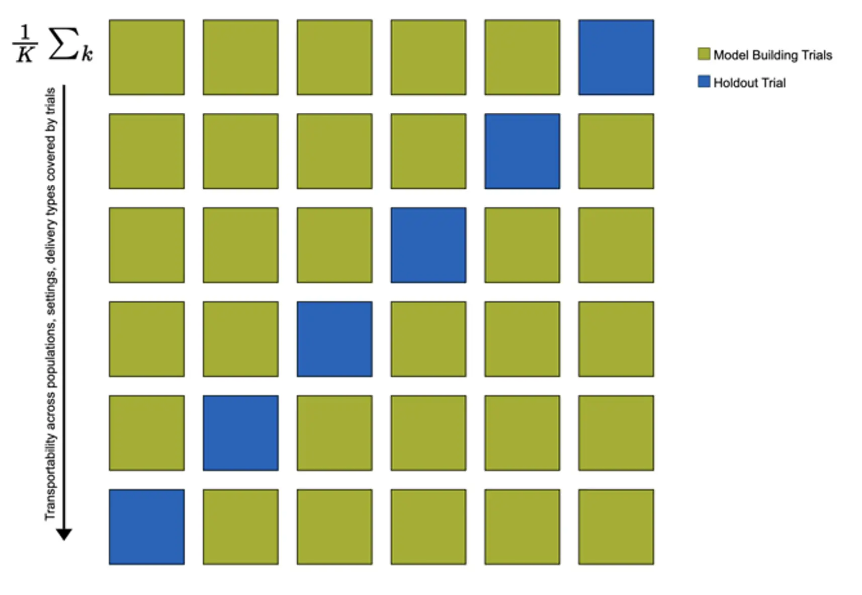
In the study, there was some variation in the studied population (case-mix), setting, and implementation of the digital stress intervention across trials. This allowed me to examine the transportability of the developed models, i.e., the potential generalizability of model predictions in populations external to those used for model development (Riley et al., 2021). I used “internal-external” cross-validation to estimate each model’s transportability. This means that models' predictive performance is estimated in $K$ cycles, where, in each cycle, one study $k$ serves as the holdout test set, while all other IPD is used for model fitting (see Figure 11 for an illustration). This method also allows us to examine potential heterogeneity in models' predictive performance across trials.

It is frequently stressed that predictive accuracy alone is not informative about the clinical utility of a prognostic model (Steyerberg, 2019; Kent, Van Klaveren, et al., 2020; Vickers et al., 2007). Predictions of predictive models should allow for improved clinical decision-making, i.e., the discrimination between future patients who do or do not benefit from the intervention. Thus, I additionally conducted a clinical usefulness analysis focusing on conditional average treatment effects (CATE; Li et al., 2018), meaning benefit scores predicted by the main models $M Baseline$ .

**Figure 11.** Schematic overview of internal-external cross-validation across $K$ studies for predictive models.

The approach I employed heavily draws on the Neyman-Rubin Causal Model (NRCM) (Aronow & Miller, 2019). Adopting Rubin’s (1974) potential outcome framework, CATEs can be viewed as estimates of the expected causal effect $τ$ of the intervention in some individuals $i$ with identical covariate values $x$ :

τ (x) = E [Y (Trt) - Y (\neg Trt) ∣ X = x]

(13)

In our case, they may be more elegantly expressed as individualized estimates of the (standardized) between-group intervention effect size, $ˆ δ i$ . These estimates can be used to assign the intervention based on a “precision treatment rule” $d c (X)$ using some clinically meaningful cut-point $c$ (Chen et al., 2017; Huling & Yu, 2018). This leads to two subgroup-conditional effects for individuals for whom the treatment is recommended ( $δ Trt$ ), versus not recommended ( $δ \neg Trt$ ):

δ Trt (d c) = E [Y | T = Trt, d c (X) = Trt] - E [Y | T = \neg Trt, d c (X) = Trt] δ \neg Trt (d c) = E [Y | T = Trt, d c (X) = \neg Trt] - E [Y | T = \neg Trt, d c (X) = \neg Trt]

(14)

We can also derive the overall benefit $δ$ of the treatment allocation rule $d c (X)$ over the entire population:

δ (d c) = E [Y ∣ T = d c (X)] - E [Y ∣ T \neq d c (X)]

(15)

It is possible to calculate empirical versions of these entities ( $ˆ δ Trt$ , $ˆ δ \neg Trt$ and $ˆ δ$ ), but they are likely to be positively biased (Athey & Imbens, 2016). Therefore, bootstrap bias correction was applied to obtain optimism-adjusted estimates of the subgroup-conditional effects (Huling & Yu, 2018). For the $lbbLMM$ algorithm, this procedure was again applied to a random subset of $m$ =5 imputation sets.

Subgroup-conditional effects were estimated based on two clinically relevant, a priori determined thresholds. First, I assumed a cut-point of $c$ =-2.40, representing the minimally important difference (MID) for depression treatment effects established in previous literature (Cuijpers et al., 2014). Assuming that most CATEs are positive, I expected this cut-point to select a patient subset for whom intervention effects are so negligible that allocation of treatment is not warranted. As a more conservative threshold, I also employed a cut-point of $c$ =−6.02 based on the reliable change index (RCI; Jacobson & Truax, 1992), which was calculated in the development data.

To be clinically useful, the precision treatment rule should assign patients with clinically relevant treatment benefits to the “treatment recommended” subgroup, while patients with clinically negligible or no treatment benefits are allocated to the “treatment not recommended” subgroup. Thus, upon implementation of the treatment assignment rule, the bootstrap-bias corrected estimate of the treatment effect/benefit in the “treatment not recommended” subgroup should be clinically negligible (i.e., too small to warrant assigning the intervention from a clinical standpoint), while the estimated effect in the “treatment recommended” group should be high.

I assumed that nearly all CATEs are positive; i.e., that patients for whom the intervention is genuinely harmful compared to no treatment are very rare or nonexistent. Therefore, for the treatment rule to be useful, estimates of its overall benefit $ˆ δ$ should be as close as possible to the unconditional treatment effect. The latter is representative of a “treat all” strategy (i.e., the expected overall effect if all patients receive the intervention), in which Equation (15) simplifies to $δ (d c) = E [Y ∣ T = Trt] - E [Y ∣ T = \neg Trt]$ .

In Article 4, algorithmic modeling was used to examine heterogeneous treatment effects of a digital intervention for depression in back pain patients. The target outcome was effects on PHQ-9 depressive symptom severity at 9-week post-test. Two RCTs were available for this study, one focusing on subthreshold depression patients, and the other on patients with a clinical diagnosis of MDD (Baumeister et al., 2021; Sander et al., 2020). The same intervention was applied in both trials. In our secondary analysis, we employed decision tree learning to detect subgroups with differential treatment effects. Our model was externally validated in a third trial among back pain patients with depression who are currently on sick leave (Schlicker et al., 2020). As before, we combined algorithms derived from machine learning with parametric multi-level models, employing “multi-level model-based recursive partitioning” (MOB; Fokkema et al., 2018). Parts of the explanations below can also be found in Harrer, Ebert, Kuper et al. (2023).

In this study, a data-driven approach was used to select relevant baseline indicators for further modeling steps. Putative moderators were entered into the random forest methodology for model-based recursive partitioning ( $mobForest$ ), as described by Garge (2013). This approach uses not one, but an ensemble of model-based decision tree learners ( $n$ =300 in our case). Splitting variables are selected randomly, resulting in more stable and less sample-specific predictions. The primary objective was to preselect a more parsimonious set of variables for the subsequent multivariate analysis (Genuer et al., 2010). In the node model, post-test depression symptoms were regressed on the treatment condition, with all potential moderators included as partitioning variables. Variables that had a positive importance index or were significant in a previous univariate moderation analysis were included as partitioning variables in the subsequent modeling steps.

Multi-level model-based recursive partitioning was then used to obtain a final decision tree predicting differential treatment effects. MOB can be applied to any parametric model fitted using $M$ -type estimators (e.g., OLS or maximum likelihood; Fokkema et al., 2021; Zeileis et al., 2008), including multi-level models as commonly used in IPD-MA. These partitioning algorithms operate on the notion that a single global model does not fit the data adequately. Using parameter stability tests, these algorithms try to determine an optimal set of splits in the data, leading to more stable sub-models in each terminal node.

In our study, the stopping rule of this process was defined by setting the significance level for parameter stability tests to $α$ =0.05, with Bonferroni-corrected p-values for pre-pruning. Cohen’s d was calculated as a standardized measure of the “individualized” effect (CATE) prediction within each terminal node subgroup. The optimism-corrected performance of the resulting tree was evaluated using the bootstrap-based correction approach by Harrell et al. (1996), with $B$ =1000 bootstrap samples.

A computational challenge in this study was that only two trials were available in the development set, which means that estimation of between-study heterogeneity variances $τ 2$ in the node models is not straightforward. Keeping with a random-effects assumption, we therefore extended the “glmertree” approach by Fokkema et al. (2018) to allow for maximum penalized likelihood (MPL)-based estimation of the node models. This method allows us to fit the multi-level IPD-MA models while introducing an additive penalty term for the (heterogeneity) variance $τ 2$ to be estimated in each node (Chung et al., 2013):

𝛃 𝛃 ℓ p (τ, β, σ ϵ; y) = ℓ (τ, β, σ ϵ; y) + log p (τ)

(16)

Where $y$ is the response variable (depressive symptom severity at 9-week post-test), $𝛃 β$ is a $p$ -dimensional vector of fixed effects, and $ϵ i k \sim N (0, σ 2 ϵ)$ is the residual for each patient $i$ in trial $k$ . It is possible to define a density for the penality function $p (τ)$ , which is equivalent to assigning a Bayesian prior on $τ$ , and facilitates the computation of the model. In our case, we imposed an inverse Wishart prior on the covariance matrix $Σ$ for the random effects of the intercept $τ α$ and treatment effect $τ θ$ :

[τ 2 α ρ τ α τ θ ρ τ α τ θ τ 2 θ] \sim IW 2 (ν, Ψ)

(17)

This adapted model was then used in the nodes while employing the recursive portioning routine.