Heterogeneity, Exchangeability & Meta-Analysis
Today, most psychiatric disorders are viewed as latent constructs identified by a collection of “characteristic” features, better known as symptoms. Commonly used diagnostic systems, including the Diagnostic and Statistical Manual of Mental Disorders (DSM-5), define mental disorders as “polythetic” constructs, i.e., as checklists of necessary and sufficient symptoms that, once fulfilled, result in a specific diagnosis (Krueger & Bezdjian, 2009; Regier, 2007). A characteristic feature for most disorder types is that some, but not all listed symptoms need to be fulfilled to make a diagnosis. For major depressive disorder, for example, the DSM-5 lists nine diagnostic criteria, only five of which need to obtain for a diagnosis to be made.
Many authors have pointed to the limitations of this classification system, which has been called a “Chinese menu”-type approach to diagnosis (Regier, 2007; Whooley, 2010). A major problem of current taxonomies is their failure to capture the, at times enormous, heterogeneity of symptom profiles within postulated disease entities. For depression, for example, there are more than 1,000 unique symptom combinations leading to a diagnosis of major depression (Fried & Nesse, 2015); for PTSD, this number is 636,120 (Galatzer-Levy & Bryant, 2013). For more than half of all mental disorders, current classification systems can lead to the paradoxical situation in which patients can receive the same diagnosis without sharing a single symptom (Olbert et al., 2014).
A further problem of the polythetic approach is that it provides all but fuzzy boundaries between diagnoses due to symptom overlap, inflating their apparent similarity, and leading to many patients fulfilling the criteria for multiple disorders (Forbes et al., 2023).
Against this backdrop, it is not too surprising that clinical heterogeneity has been found to be a defining feature of many mental disorders, ranging across patients, populations, and age groups (Fried & Nesse, 2015; Goldberg, 2011; Nandi et al., 2009; Steinhausen, 2009).
Following Nunes et al. (2020b), this clinical heterogeneity can be viewed as a type of multimodality: existing disorders classifications are, in fact, sets comprised of many distinct clusters that appear with relative abundance, but cannot be differentiated a priori in a robust or reliable way. In part, this ignorance may be a logical consequence of the polythetic approach itself, which maintains to be “etiologically agnostic” for most disorders; i.e., not based on a single well-defined pathogenic pathway, which is often unclear (Castiglioni & Laudisa, 2015; McLennan & Braunberger, 2018). This relates to the often-stated equifinality of mental illness, whereby a wide range of developmental pathways can lead to one and the same disease phenotype (Cicchetti & Rogosch, 1996); as well as multifinality, which describes the reverse case. Kendler (2021) brings the problem to the point:
“We assume that constructs, such as schizophrenia or alcohol use disorder, exist but we can only observe the signs, symptoms, and course of illness that we postulate result from these disorders. Despite years of research, we cannot explain or directly observe the pathophysiologies of major mental health disorders that we could use to define essential features. […] [A] major criticism of our current nosologic efforts has been the limited progress made in moving from descriptive to etiologically based diagnoses.”
Kendler also alludes to issues we discussed above: in lack of a clearly identifiable causal pathway to define what is “real” about a mental disorder, and left with all but a descriptive analysis of “congeries of symptoms” (Hacking), existing taxonomies have to be seen as no more than preliminary. He states that:
“While reality is an unforgiving criterion, empirical adequacy is more flexible, can be progressively improved upon, and is subject to varying constructions. […] Indeed, Emil Kraepelin, was tentative in his diagnostic conclusions, experimenting with various nosologic categories over his career, and repeatedly revising earlier formulations. Furthermore, near the end of his life, he proposed several quite different approaches to conceptualizing psychiatric illness, the most famous being that of an organ register. […]
Anyone familiar with the history of psychiatry can name many diagnoses, popular at earlier times (eg, monomania, masturbatory insanity, hysteria), that have since been rejected. Even ardent DSM advocates are unlikely to claim that all current diagnoses are the final word.”
Heterogeneity of Treatment Effects
Heterogeneity is not only a defining feature of mental disorders, but also characteristic of how many patients respond to psychological treatment. “Heterogeneity of treatment effects” (HTE) is often used as an umbrella term to describe that not all patients profit in the same way from each psychological intervention. This is often taken as a sign that informed treatment selection could optimize the outcomes of individual patients (Cohen et al., 2021; Kent, Paulus, et al., 2020). From a methodological perspective, HTE presents itself as a multi-faceted problem, requiring differentiation between two distinct layers of investigation.
For once, patients may genuinely respond differently to the same intervention, in the sense of showing distinct individual treatment effects (ITE). Such ITEs are defined by counterfactual information, and are therefore not directly observable. However, based on data from, e.g. RCTs, one may identify sets of patient-level markers that predict conditional average treatment effects (CATE). CATEs, which can be derived from the Neyman-Rubin causal model (NRCM), will be covered in greater detail in the methodological innovation section. If CATEs differ substantially for the same intervention, this implies some degree of effect modification: the treatment is more effective for some patients, and less effective for others.
Given certain assumptions (to be covered later), identification of HTE is straightforward – at least theoretically. In practice, however, we are faced with the problem that HTE has to be estimated from some specific context (e.g., some trial or study), while our inferential goals are typically much broader. It is, for example, much more likely that researchers will be interested in differential effects of some treatment in general, not in HTE of a specific treatment observed in a specific trial, or a particular setting, at some point in the past. This adds a second layer of heterogeneity, associated with the specific context in which a treatment is provided, and with the particular research methodology that was applied in a study.
The most trivial example is case-mix heterogeneity, whereby trials (or sites, clinics, etc.) may have recruited different subsets of patients (e.g. patients with more severe symptoms, older patients, more females, etc.). If recruited patient groups differ on relevant effect modifiers across sites, this will lead to different average treatment effects (ATE) in each context, even if exactly the same intervention was used. In psychotherapy research, matters are often even more complex, beginning with the provided interventions themselves.
Even if purporting to implement the same format (i.e., CBT for depression), psychological treatments are far from standardized. They can also be provided in different intensity, varying formats (individually, group-based, online), and their quality may differ depending on the “allegiance” or qualification of their providers (Munder et al., 2013; Harrer, Cuijpers, et al., 2023). For most treatments, therapist effects also add another level of variation (Wampold & Owen, 2021; Magnusson et al., 2018). All of these factors may plausibly manifest themselves in differential treatment effects.
If treatment effects are to be obtained from RCTs, a suite of other methodological context factors have to be added to this list, including the type of comparator used (Michopoulos et al., 2021), or the study’s overall risk of bias (Cuijpers, Karyotaki, et al., 2019). Measurement differences may be yet another, albeit often omitted concern (Sprenger et al., 2024).
This creates a hierarchy of patient and context-related effect modification, whereby both levels may also interact with each other: for trials, a specific case-mix may also predict certain methodological particularities. In meta-analyses, this “web of confounding” reappears in an amalgamated form, where only aggregated effect sizes are typically available for further analysis. Figure 3 visualizes this relationship.

Meta-analytic evidence shows that psychological treatment effects are often highly heterogeneous. This includes both between-study heterogeneity, as commonly estimated in random-effects models (Cuijpers, Miguel, Harrer, et al., 2023; Cuijpers et al., 2024; Harrer, Miguel, et al., 2024), as well as meta-analyses of variance ratios (VRs; Kaiser et al., 2022; Terhorst et al., 2024), indicating that HTE may also exist on a participant level. The latter finding is in contrast to similar studies in antidepressants and antipsychotics, were participant-level HTE is less certain (McCutcheon et al., 2022; Plöderl & Hengartner, 2019; Winkelbeiner et al., 2019).
For both “layers” of heterogeneity, true causes for this variability are largely unknown. We are yet to determine robust participant-level effect modifiers for psychological treatment (save, potentially, for initial symptom severity; Cuijpers et al., 2022; Schneider et al., 2015; Sextl-Plötz et al., 2024). While some study-level characteristics typically predict differential treatment effects in meta-analysis (e.g. risk of bias or type of comparator), these indicators are often insufficient to appreciably reduce the enormous amount of between-study heterogeneity detected in meta-analytic psychotherapy research (see, e.g., Cuijpers et al., 2007; Cuijpers, Harrer, Miguel, et al., 2023).
This is a troubling observation. Meta-analytic point estimates currently make up the top of the “evidence pyramid” (Guyatt et al., 1995), and build the basis for treatment guidelines and other forms of policy making. Yet, under strong heterogeneity, these “averages” may be largely meaningless, having hardly any predictive value pertaining to the effect of a specific treatment, in a specific patient, in a specific context. We will return to this fundamental generalizability problem later.
To illustrate the true impact of heterogeneity on the cross-contextual variability of treatment effects, we employed a method proposed by Mathur and VanderWeele (2019). Using empirical estimates of between-study heterogeneity across 12 mental health problems, we plotted the true effect size distribution of psychological treatments. These distributions were centered around the meta-analytic point estimate for each indication, and we highlighted the proportion of true effects that are either clinically negligible, or even indicate harm. These illustrations are based on the simplifying assumption that true effects follow a normal distribution, and they only refer to variability on a study level.

Despite this limitation, the plots depicted in Figure 4 allow to gauge how strongly, based on present evidence, the effects of psychotherapy truly differ across contexts. Large parts of the distributions indicate settings in which the true treatment effect is clinically negligible, or even negative; even though the pooled effect (vertical line) is positive and significant throughout. On the other hand, there are also settings displaying much higher effects than the pooled average.
A Formal Definition of Heterogeneity
In the previous two chapters, we have examined heterogeneity in mental disorder classifications, as well as in patients' response to psychological treatment. We have done so without yet providing a formal definition of what “heterogeneity” actually signifies. The term is frequently used in the medical literature, but typically without any further conceptual elaboration. As “clinical” heterogeneity, it may refer to some true variability or diversity within endotypes, populations, study designs, treatment effects, data sets, and so forth (Altman & Matthews, 1996; Fletcher, 2007; Higgins & Thompson, 2002). This word-use needs to be distinguished from heterogeneity in statistics, i.e., as an identifiable quantity (e.g., a variance component) that we want to estimate from a set of data.
Looking at our examples above, we see that heterogeneity can take on quite distinct forms. In mental disorder classifications, heterogeneity manifests itself if an entity is comprised of many sub-classes (i.e., “presentations”) that appear with some level of abundance. Following Nunes, Trappenberg and Alda (2020b), we call this “heterogeneity-as-multimodality”. This is juxtaposed to heterogeneity as manifested in HTE, i.e., as variability on some continuous measure, which we term “heterogeneity-as-deviance” (ibid.). A common thread across both conceptualizations is that there is some degree of variability within a system that cannot, as of now, be fully explained or predicted. This implies that heterogeneity limits our ability to make generalizable scientific inferences (Bareinboim & Pearl, 2016).
Despite its prime importance, there is no overarching formal framework on how heterogeneity can be best conceptualized and measured in psychiatric research. Towards a more formal definition, we will therefore trace back pioneering work put forward by Nunes, Trappenberg and Alda (2020a; “NTA” in the following). The indicators we introduce are based on information theory and have been used in other fields, such as ecology, for many years. This framework offers some heuristic value, particularly in linking the concepts of “heterogeneity-as-multimodality” and “heterogeneity-as-deviance” through information-theoretic “numbers equivalent” measures.
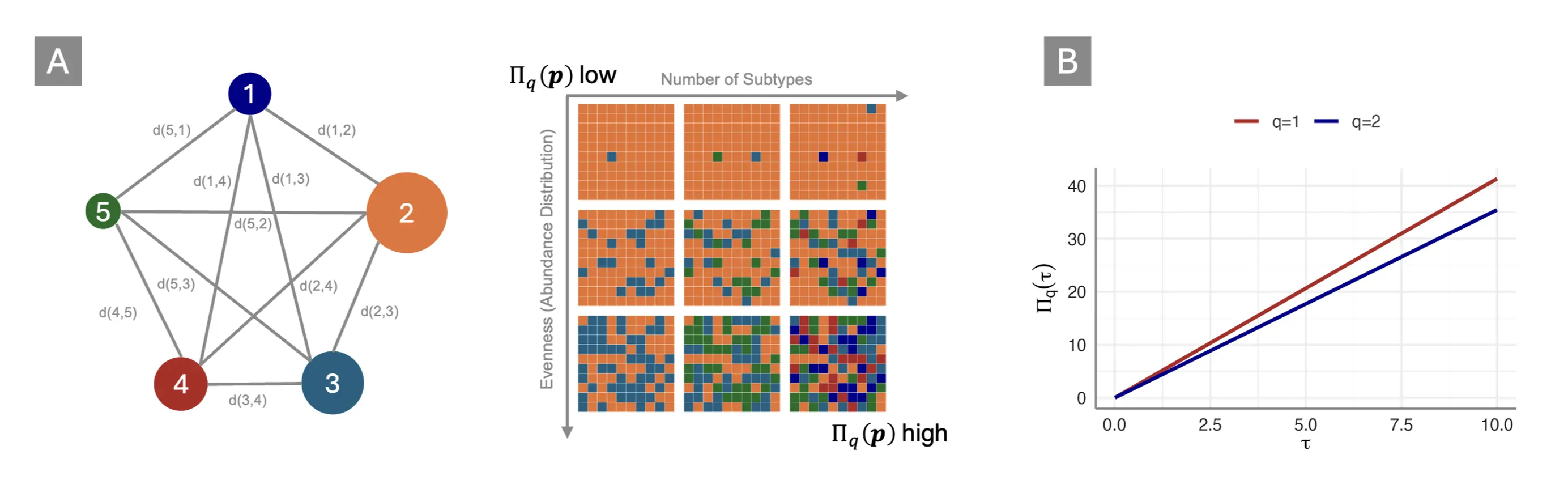
We begin with our categorical “heterogeneity-as-multimodality” subtype. Suppose we are to examine some system or entity $\mathcal{S}$; for example, “major depression” as defined by the diagnostic criteria of the DSM-5. Heterogeneity (i.e., the absence of perfect conformity) implies that $\mathcal{S}$ is a mathematical set or “sample space” of distinct potential observations $\mathcal{S}=(s_1,s_2,\ldots,\ s_n)$ (in our case, these observations or elements s represent distinct “presentations” of the disease).
Overall, $\mathcal{S}$ can be defined by the distance $d\left(s_i,s_j\right)$ between any two elements $s_i,\ s_j\in\ \mathcal{S}$; as well as the relative abundance of each element. If these abundances sum up to 1 over $\mathcal{S}$, its elements follow a probability distribution $P\left(s\right)$. Since $\mathcal{S}$ is a categorical system, the distance function $D$ can be defined as follows:
i.e., the distance is constrained to 1 for each set of distinct elements, and to 0 for identical elements. A straightforward measure to describe such a system is the number of unique symptom combinations, like the number of unique profiles for major depression and PTSD we referenced in the last chapter. This number can be computed like so, with $N$ being the total, and $K$ being the minimum number of symptoms needed to fulfill the diagnostic criteria of a disorder:
NTA argue that such combinatoric approaches are inappropriate to capture heterogeneity in a system, since they fail to account for the relative abundance of different elements: a system may still be fairly homogeneous if one particular presentation dominates the system, even if the total sample space is large. They instead propose measures derived from the Rényi entropy, $H_q(\boldsymbol{p})$ (Bashkirov, 2006):
where $p_i$ is the probability of the ith presentation within a given system. The Rényi entropy is a generalized measure depending on the q parameter. When $q\rightarrow0$, we obtain the support of a system; i.e., we return back to the log-number of distinct elements in $\mathcal{S}$:
Using L’Hôpital’s rule, we can also calculate the limit for $q\rightarrow1$, which yields the commonly employed Shannon entropy (Shannon, 1948, chap. 6):
Lastly, the collision entropy obtains when $q\rightarrow2$:
The crucial step to turn these entropies into heterogeneity measures is to apply the exponential function to them. This yields a generalized family of “Rényi-type” heterogeneities $\Pi_q\left(\boldsymbol{p}\right)$, displaying the effective number of distinct elements in a system. Except for the limiting case of $q\rightarrow0$, $\Pi_q\left(\boldsymbol{p}\right)$ measures account for both the number of distinct elements or classes in a system, and the relative abundance with which they appear. This relationship is visualized in Figure 5, Panel A below. Therefore, they can be used be used to gauge how much a given system diverges from a state of perfect conformity, i.e., how much heterogeneity it displays.
This way we can, for example, transform the Shannon entropy in Equation (5) into a measure of perplexity, $\Pi_1\left(\boldsymbol{p}\right)=e^{-\sum_{i=1}^{n}p_i^\ \log_e{p_i}}$, the effective number of typical categories in a system. Units of Rényi heterogeneity can be understood as the number of classes a “hypothetical” system with perfectly even class distribution would require to be just as heterogeneous as the system under study. Given that classes (i.e., symptom presentations) typically do not appear equally often, these “numbers equivalent” will be lower than the total number of possible presentations in almost all cases. Intuitively, the Rényi heterogeneity can thus be understood as the number of “equally common” presentations in a system. This value provides a yardstick to compare the “true diversity” (Jost, 2007) of two or more systems.
As of now, these indices presuppose a categorical system, and we have omitted “heterogeneity-as-deviance” as it arises, for instance, in treatment effects. In the supplement (p. 26ff.), NTA try to fill this gap by extending Rényi heterogeneity to systems with continuous data. In particular, they attempt to show that “numbers equivalent” are linked to the between-study heterogeneity variance $\tau^2$ as estimated in random-effects meta-analyses. Using an extension of the Rényi entropy for the normal distribution, it is shown that:
This leads to $\Pi_1\left(\tau\right)$ as a measure of the “effective number of typical study effects”, or $\Pi_2\left(\tau\right)$ as the “total number of common study effects”. Panel B in Figure 5 depicts this relationship, showing that $\Pi_q\left(\tau\right)$ increases linearly along with $\tau^2$. A potential drawback of these indices is that $\tau$ is scale-dependent, while $\Pi_q\left(\tau\right)$ is not; “studies equivalent” would therefore depend on the outcome measures chosen as part of the meta-analysis.
The “numbers equivalent” measures defined above are a promising method to formalize heterogeneity within a single overarching framework. This, however, does not obliterate the need to define the level of analysis on which heterogeneity manifests itself (Nunes et al., 2020b). In the categorical case, the formulas above assume that mental disorder classifications are formed by “atomistic” subtypes that are (i) clearly distinct from other presentations, and (ii) cannot be differentiated any further. While this may be fairly trivial for, say, biological species, it may cause all kinds of conceptual complications for mental disorders. In our case, presentations are combinations of “symptoms”; where the latter are not unambiguously defined, often highly intercorrelated, and typically not directly measurable.
In terms of HTE, we already mentioned that heterogeneity appears on different layers. In meta-analysis, the focus is typically on the individual studies, meaning that heterogeneity manifests itself, and is quantified on, this “layer”. We covered that this approach is reductionistic, in the sense of making studies (or sites, contexts, etc.) the unit of analysis, while the true underlying mechanism causing differential treatment effects operates on several interlocking layers (e.g. participant and context-related factors, which may interact with each other).
It is important to emphasize that formalization of heterogeneity alone will not be sufficient to understand its impact on the generalizability of our findings. In the following chapter, we will therefore examine what heterogeneity means for our ability to make robust scientific inferences. We will do so by first delving deeper into heterogeneity as captured by the meta-analytic model. We will see that the latter is part of a general family of multi-level models, ubiquitous in quantitative social science, and connected by the assumption of random effects. The statistical concept underlying these models is exchangeability, which encodes our own ignorance concerning the true causes of variability in a sample. Lastly, we will consider arguments that random effects, if applied “honestly”, highlight serious limitations in the utility of quantitative psychotherapy research.
Heterogeneity & Exchangeability
One of the most common ways to capture heterogeneity statistically, i.e. as part of a parametric model, is through the use of multi-level models (MLMs). These models appear under different names in the literature, including “hierarchical models”, or “mixed models”. Meta-analysis belongs to this broad model family (Pastor & Lazowski, 2018), and some structural equation models (SEMs) can be reformulated as MLMs as well (Harrer et al., 2021, chap. 11). MLMs are a truly pervasive model type; while the exact terminology and implementation may vary across fields, they remain heavily used in various disciplines, including ecology (Bolker et al., 2009), public health (Diez-Roux, 2000), economics (Gelman & Hill, 2007), social science (Raudenbush & Bryk, 2002), or biomedicine (Brown & Prescott, 2014).
All MLMs share the idea that several parameters in a model can be regarded as “related”, meaning that a joint probability distribution can be assumed to reflect their dependence (Gelman et al., 2021; p. 101). MLMs allow for variability in the true value $\theta_i$ of each unit $i$ in our analysis, by conceptualizing them as “random effects”. These random effects occur because all $\theta_i$’s are seen as samples from an overarching population distribution or “superpopulation”. If we conjecture (as is often done) that this population distribution is normal, the random effects can be described succinctly by the grand mean $\mu$ of the superpopulation, and its variance $\tau^2$. The latter quantifies how variable the true values are, i.e., it is a reflection of the heterogeneity displayed by our sample. In random-effects meta-analysis, the estimation of $\tau^2$ is therefore a crucial step to quantify the robustness of a pooled value: as $\tau^2$ grows, the summary effect becomes less and less representative of the true outcome variability we want to generalize across.
For now, let us assume that a normal distribution $\mathcal{N}\left(\mu,\sigma^2\right)$ indeed appropriately describes the data-generating mechanism giving rise to “random effects” in some analysis of interest. This yields a “normal-normal” hierarchical model $\mathcal{M}^{NN}$, which we can denote like this:
We see that this assumes sampling processes on two levels: one within units $i$ (e.g., within studies); and one between them. On the first level, it shows that the measured value $y_i$ recorded for each unit is a mere reflection of its true value $\theta_i$, whereby $y_i$ differs from $\theta_i$ due to sampling error. However, sampling error alone cannot fully explain the variation in our data: there are real differences between units in their true value $\theta_i$; they are different but assumed to be related, because they are drawn from the same super-population of true values. In meta-analysis, the goal is typically to estimate the mean or expected value $\mu$, defined by the second “layer” in Equation (8).
Many meta-analytic approaches make the same assumptions as we did in defining $\mathcal{M}^{NN}$; i.e., that true values follow a normal distribution. In reality, this assumption is not necessary, and often incorrect (Higgins et al., 2009; Jackson & White, 2018; Liu et al., 2023; Noma et al., 2022). In fact, from a Bayesian perspective, we only need to assume that the true values $\theta_i$ are generated by some mechanism $f\left(\phi\right)$, parameters $\phi$ of which are unknown, but can be given a prior distribution1Technically, we say that the true values $\theta_i$ are independent and identically distributed (i.i.d.) after conditioning on $f\left(\phi\right): \theta_i|\phi$..
Exchangeability is a corollary of Bruno de Finetti’s (1906-1985) representation theorem (Heath & Sudderth, 1976; Bernardo, 1996; Diaconis & Freedman, 1980). This theorem itself is a foundational concept in probability theory, while exchangeability has been called the “fundamental assumption of statistics” (Greenland, 2008). It is grounded in a subjectivist interpretation of probability, which, through the likes of Frank P. Ramsey (1926), Leonard J. Savage (1972), or Dennis Lindley (2000) has paved way for the “rebirth” of Bayesian statistics in the later 20th century (Senn, 2023, p. 84ff.). This interpretation holds that probability is an opinion, i.e., a bet a person makes about events or a parameter (Greenland, 2008). This personalized probability is not detached from “reality”, in the sense that new experience can be used to update it: as new evidence is incorporated, probabilities p assigned by different persons will converge to a similar value over time. I quote Savage (1972, p. 68):
“[I]n certain contexts any two opinions, provided that neither is extreme in a technical sense, are almost sure to be brought very close to another by a sufficiently large body of evidence.”
The main requirement is that subjective probabilities are coherent: they need to follow basic axioms of probability theory, and must not contradict themselves (Senn, 2023, p. 85). Exchangeability is related to this concept. Formally, we can say that a sequence of random variables, e.g., some true effects $p\left(\theta_i,\ \ldots,\ \theta_k\right)$, is exchangeable when its joint probability is identical under any permutation of the subscripts $\pi$:
i.e., the joint distribution remains the same under any “re-ordering” in which the elements appear (for example over time). This assumption is central because it states that information from each true effect is treated in exactly the same way, no matter where it appears in the sequence. This expresses the symmetry of our beliefs: the values of different $\theta$’s may differ, but there is nothing in our knowledge to further distinguish between them (Gelman et al., 2021; p. 105; Schervish, 1995, chap. 1.2).
It is important to emphasize that exchangeability does not require the true values to all be independent of each other; in fact, there are many plausible cases where this is highly unlikely. In meta-analysis, for example, earlier studies may have influenced trials that were published more recently, and there are probably many other ways in which studies may be related. The core idea is that we, from a subjective standpoint, assume these values to be a priori exchangeable. This is because we have no information that could allow to differentiate between them.
Random effects, so often used for statistical modeling across various disciplines, thus do not encode much more than our own ignorance: it is assumed that true values are different-but-similar, yet in ways we do not understand, and cannot predict as of now. Gelman and colleagues (2021, p. 104) state this succinctly:
“In practice, ignorance implies exchangeability.”
As discussed, this prior ignorance on real variability and its causes is a defining problem in psychotherapy research. Deeper inspection of the exchangeability assumption reveals that supposition of random effects, as often done in research, cannot “explain away” this fundamental issue. At best, it helps to quantify our own ignorance about the true variability in effects, and our inability to predict them.
It is important to emphasize that, from an inferential perspective, random effects still fulfill an important purpose. Modeling heterogeneity via random-effects is “costly”, in the sense of leading to broader confidence intervals, and even broader prediction intervals. This behavior is intended, given that random-effects models do not condition on the true effects or outcomes at hand; instead, true values $\theta_i$ are seen as random instances of a hypothetical “superpopulation”. The goal is therefore to provide unconditional inferences that incorporate and, more importantly, generalize over all true effects (Hedges & Vevea, 1998).
The “Generalizability Crisis”
Random effects are also used as a didactic device in Yarkoni’s (2022) “generalizability crisis”; a landmark paper arguing that the context-sensitivity displayed by psychological phenomena renders most quantitative research all but pointless. Yarkoni’s critique centers on a fundamental mismatch between inferential goals in psychological research, and the concrete studies from which they are drawn. Most psychological theories and hypotheses are articulated verbally, in the form of “law-like” relationships intended to generalize over a broad range of contexts. Many examples from the history of psychology could be named here, such as the “frustration-aggression hypothesis” (i.e., that frustrated people tend to be more aggressive; Berkowitz, 1989) or “cognitive dissonance” (i.e., that humans strive for consistency between their beliefs and actions; Harmon-Jones & Mills, 2019).
Similar claims are also made in psychotherapy research, where we stipulate that some treatment $T$ “works”; or that two treatments $T^{\left(1\right)}$ and $T^{\left(2\right)}$ are “equally effective”. It is assumed that such hypotheses can and should be tested quantitatively, i.e., using a numeric measure of the outcome, and a concrete operationalization of the construct we want to test. Optimally, instances of the “independent variable” are assigned randomly to participants, to “prove” the causal claims implied by the hypothesis. Randomized controlled trials can be seen as a subtype of this research design, which dominates large parts of modern psychology.
Yarkoni is not criticizing randomization as a method for obtaining internally valid, causally interpretable evidence, but rather the “sweeping verbal generalizations” that studies are taken to support. His central point is that quantitative studies are restricted not only because they involve a small sample of participants, but also because very broad hypotheses are operationalized in a very specific, narrow way to make the investigation feasible. In experimental research, for example, it is impossible to test all possible stimuli, settings, and contexts under which humans may be “frustrated” and to examine the effect on aggression (which can be measured in countless different ways as well). Each study will, therefore, only represent a random instance of how a phenomenon can be operationalized. At the same time, even minor changes in the operationalization could profoundly impact the study’s results.
We discussed that random effects are a method to encode our own “ignorance” about such true variation. Indeed, random effects are frequently used in psychological research to model different stimuli as mere “examples”, taken from a much larger universe of operationalizations. In meta-analytic psychotherapy research, the same logic applies to individual trials, which are assumed to be random draws from a “super-population” to which we want to generalize.
Yarkoni’s critique is that such models are still “underspecified”: sensible researchers might account for one or two random effects in their analysis (e.g., for patients, or different sites); but never for all layers of variation we actually want to generalize over. For psychological treatment studies, for example, we certainly want to generalize over minor treatment variations, differences in personnel, care as usual, research sites, therapist effects, seasonal influences, cultural determinants, time, and so forth. Many of these contextual factors will not be measured, or even known.
This, Yarkoni argues, makes it impossible to truly account for the broad “generalization intentions” we have as researchers. If we were to account for them, “a huge proportion of the quantitative inferences drawn in the published psychology literature is so weak as to be at best questionable and at worst utterly nonsensical” (Yarkoni, 2022, p. 8). Since the true variation caused by these unmeasured “layers of heterogeneity” is not known, Yarkoni himself turns to simulation, showing that even conservative estimates of $\sigma^{\textsf{unmeasured}}$ would lead to confidence intervals so broad that even a huge study “tells us essentially nothing” (ibid., p. 7).
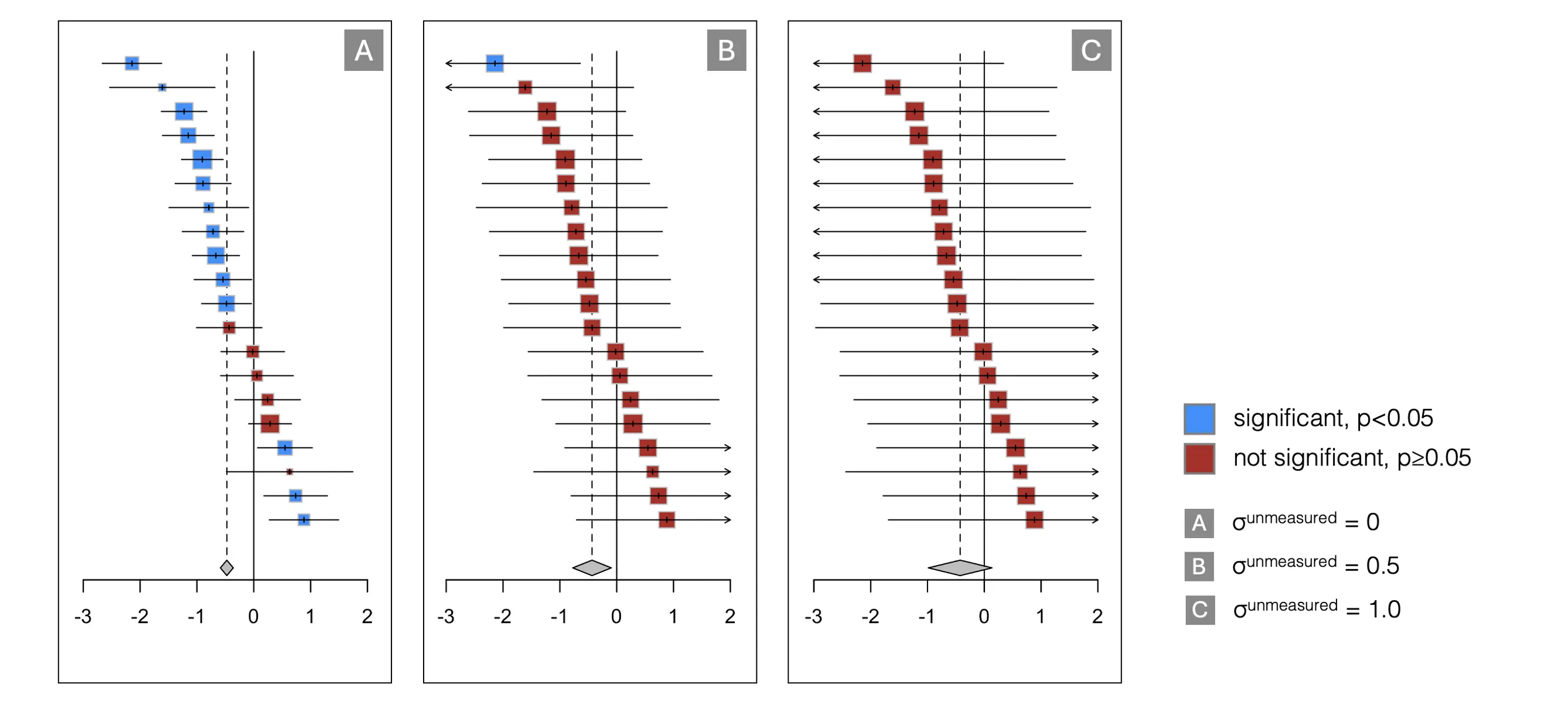
We conducted a similar Monte Carlo simulation to illustrate this problem (see Figure 6 above). Our results show the effect of $\sigma^{\textsf{unmeasured}}$ in a meta-analytic context, presuming the goal is to synthesize the effect of some psychological treatment. The graphs above show that, even when assuming a conservative estimate of $\sigma^{\textsf{unmeasured}}$ = 0.5 (roughly equal to heterogeneity variance due to study effects alone), most individual trials in a meta-analysis are rendered non-significant (Panel B). For $\sigma^{\textsf{unmeasured}}$ = 1, statistical significance cannot even be ascertained for the pooled effect anymore, assuming a common-effect model (Panel C); even though the initial estimate was highly significant (see Panel A).
This simulation can be seen as a way to visualize the true “costs” of heterogeneity, and how little quantitative investigations may contribute if generalizable findings are to be drawn complex, context-specific phenomena. As we examined in preceding pages, such problems are no less acute in psychotherapy research. Yarkoni argues that generalizability is the root cause of most “ailments” in psychological research, as its methods fail to capture the enormous variability of most entities under study (2022, chap. 5). The main argument we developed before is similar, suggesting that this context-sensitivity is integral to the matter, being deeply ingrained in the presentation of most mental disorders, and how patients respond to psychological treatments.
Thus, the central notion of this dissertation is straightforward: to make progress in psychological treatment research, we need to master heterogeneity more effectively. In the following chapters, we will elaborate on the methodological innovations examined to this end, as well as their theoretical underpinnings. Before that, a more precise delineation of our research goals is in order.